When developing a web app with a strong focus on data analysis, it’s essential to have a spreadsheet tool that not only covers most of your project’s functional requirements but also provides a smooth user experience. However, all functional capabilities of such tools can be less effective without usability features. Striking the right balance between functionality and usability is the core idea behind the new release of DHTMLX Spreadsheet 5.2.
This update introduces improvements aimed at making our JavaScript Spreadsheet component both more robust and user-friendly. On the functional side, it adds new ways to work with rows and columns, including options to hide and freeze them via the UI or API. From the usability perspective, the new version delivers visual styling for borders in selected groups of cells and formula descriptions that guide users during data entry. In addition, there is also a new event for indicating data import completion.
Let’s delve into the details.
Extra Manipulations with Rows and Columns
DHTMLX Spreadsheet is known for being flexible in terms of the table’s structural organization. Our Spreadsheet already include plenty of operations that can be done to adjust the spreadsheet structure for more effective data right from the UI. In v5.2, we expanded the arsenal of available operations for columns and rows:
From now on, any number of columns and rows in a spreadsheet can be hidden via the corresponding option in the cells’ context menu or via the toolbar buttons. Hidden elements will be marked with horizontal and vertical arrows for columns and rows respectively. If needed, a single click on these arrows will make the required elements visible again.
 Check the sample >
Previously, you could freeze columns and rows via the API only. For v5.2, our team decided not only to rewrite this functionality for developers’ convenience, but also to bring it to the UI side, opening the opportunity to easily freeze or unfreeze any number of rows and columns on the fly. It can be done via the Edit menu, toolbar buttons, and cells’ context menu.
 Check the sample >
In both samples above, we showed how to hide and freeze columns and rows using the context menu, while other options for performing these operations are fully covered in the user guide.
From a developer’s perspective, performing hide and freeze operations via the API involves using new methods, which are thoroughly described in the developer guide.
With freezing and hiding options at hand, developers and end-users gain greater control over data presentation in the spreadsheet. This contributes to more convenient comparison and analysis of information, which can be vital in data-heavy apps.
Multiple Border Styling Options
Spreadsheets often contain large volumes of data with varying degrees of relevance and importance. Therefore, it is helpful to highlight certain parts of the table to make them more noticeable. It is especially useful in collaborative environments, where this styling novelty can help draw users’ attention to important pieces of data in large tables and keep everyone on the same page.
The updated DHTMLX Spreadsheet allows making styling adjustments to borders of a selected cell or group of cells. With this feature, it becomes easy to visually separate and highlight specific data blocks, improving the readability and informative value of spreadsheets.
There are plenty of border styling options available via the corresponding toolbar button of the Spreadsheet UI. For instance, you can specify which borders from the selected cell (group of cells) should be modified (all, top, right, etc.) and play around with the color and style settings.
 Check the sample >
Whether you’re preparing a budget plan, sales report, or even a financial dashboard, this visual enhancement will boost the user experience with tabular data.
Formula Description
Remembering the purpose of all formulas is an overwhelming task even for Excel experts, let alone ordinary users. DHTMLX Spreadsheet 5.2 becomes more user-friendly in this regard by introducing a formula pop-up description. This feature provides real-time assistance by displaying descriptions of formulas in a pop-up as users start typing a formula. It will give users hints on the proper usage of any unfamiliar function supported by our Spreadsheet.
 Check the sample >
Under the hood, the pop-up description is implemented with the new formulas locale. Here is a piece of the default locale for formulas in code:
AVERAGE: [
[
"Number1",
"Required. A number or cell reference that refers to numeric values."
],
[
"Number2",
"Optional. A number or cell reference that refers to numeric values."
]
],
// other descriptions for formulas
};
If needed, it can be replaced with a custom locale via the dhx.i18n.setLocale() method:
AVERAGE: [
["Zahl1", "Erforderlich. Eine Zahl oder Zellreferenz, die sich auf numerische Werte bezieht."],
["Zahl2", "Optional. Eine Zahl oder Zellreferenz, die auf numerische Werte verweist."]
],
// other descriptions for formulas
};
dhx.i18n.setLocale("formulas", de);
Find more details in the localization guide.
Indicating File Import Completion
And lastly, we want to mention that the new Spreadsheet version ensures more reliable transfer of spreadsheet data between the web app and external files like Excel or CSV with the new AfterDataLoaded event. It will fire once the spreadsheet is fully imported into the required format and display the message after the operation is completed.
dhx.message({
text: "Data successfully loaded into Spreadsheet!",
});
});
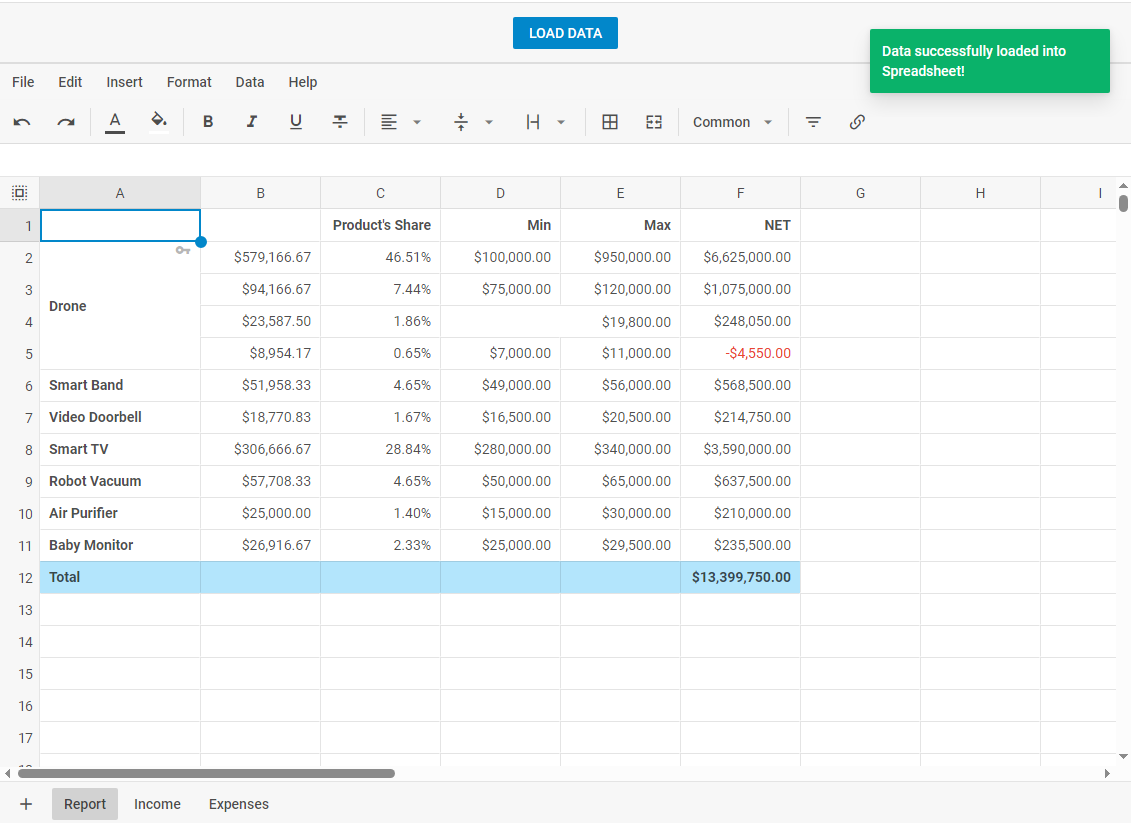
This event will be great for importing large datasets, signaling when it is safe to start calling methods for searching, filtering, etc.
That’s all about the new features included in this minor update of DHTMLX Spreadsheet. Check the “What’s New” section to make sure you haven’t missed anything. Also, do not forget to take a look at migration notes to v5.2.
If you need to test the new version of our Spreadsheet before adding it to your project, download a free 30-day trial version. Current customers can access DHTMLX Spreadsheet 5.2 via their Client’s Area.