Our whole team is thrilled to announce the release of DHTMLX Spreadsheet 5.0. This major update is primarily focused on expanding the list of capabilities for modifying the spreadsheet structure on the fly and managing tabular data with ease. For instance, the new version of our JavaScript spreadsheet library allows searching and filtering data, merging and splitting cells, automatically adjusting column width of the table, inserting links into spreadsheet content, applying the strikethrough text formatting, and more. Almost all these highly anticipated features are available via API and UI.
Let us have a closer look at how the novelties delivered in v5.0 can be used by both web developers and end-users.
Download an evaluation version of DHTMLX Spreadsheet v5.0 >
Data Searching
Finding specific pieces of data in spreadsheets may be time-consuming if you don’t have a special search tool for this task. It is especially true for large tables with multiple sheets containing hundreds or even thousands of records. But you won’t have to worry about that when using the latest version of our JavaScript Spreadsheet since it comes with a handy search option.
End-users can perform this operation via a search bar, which is opened in two ways:
- by clicking on any spreadsheet cell and pressing the Ctrl (Cmd) + F combination,
- by going to Data -> Search in the menu section.
It should be noted that the search is performed only within the opened worksheet. All the results will be highlighted right in the grid and can be reviewed using search bar arrows or hotkeys Ctrl (Command) + G (previous) / Ctrl (Command) + Shift+ G (next). By default, all searches are case-insensitive.
To find certain information in the spreadsheet via API, you have to use the newly added search() method. It takes 3 optional parameters:
- text – specifies a search value,
- openSearch – if set to true, opens the search box and highlights the results that match the entered query (false by default),
- sheetID – serves to identify the sheet where searching should be performed. If you do not set the value for this parameter, the search will be performed on the currently active sheet.
For example, you can find all income statistics for February in the corresponding sheet in the following way:
There is also the new hideSearch() method that closes the search bar:
Data Filtering
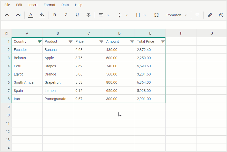
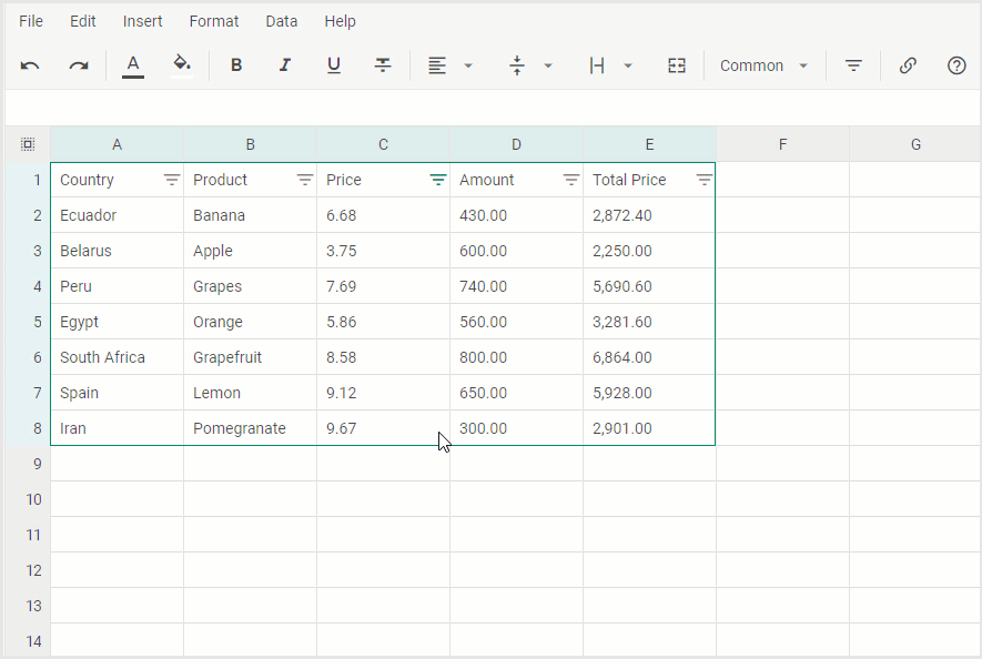
One more significant improvement for effective working with large spreadsheets provided in v5.0 is the ability to filter data by certain criteria. This feature will help you to temporarily hide cells with excessive information and concentrate on currently relevant data for more productive analysis.
In the user interface, this feature can be brought into action by selecting one or several cells and doing one of the following:
- clicking on the Filter button in the toolbar,
- going to Data -> Filter in the menu section.
After that, selected cells or ranges of cells will be complemented with filter icons. Then it is possible to start filtering data by condition or by value.
When filters are no longer needed, end-users can remove them by clicking on the Filter button in the toolbar or on the corresponding option in the Data menu of the spreadsheet. As a result, all hidden records will become visible.
Here are visual examples that show step by step how to filter data both ways and clear filtering settings afterward:
- Filtering by condition
- Filtering by values
When talking about implementing data filtering via API, you should call the setFilter() method.
It enables you to set a cell or range of cells to be filtered and add certain rules that should be followed during this operation.
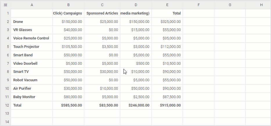
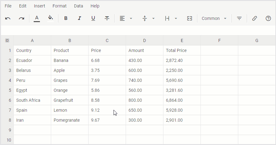
For instance, you can display cells in column C, where numeric values are not between 5 and 8, excluding 3.75 like in the example below:
Now let us consider how to use the setFilter() method for specifying the filtering criteria for two columns using the following example:
In this case, the first condition, namely “between 5 and 8”, is applied to column C, while the condition for excluding 740 works for column D.
The full list of available conditions for filtering and their meaning are provided in the documentation.
To reset the filter, you need to call the setFilter() method, indicating only the first cell parameter or without specifying any parameters at all.
If necessary, you can get the criteria that are currently used for filtering spreadsheet data with the help of the getFilter() method.
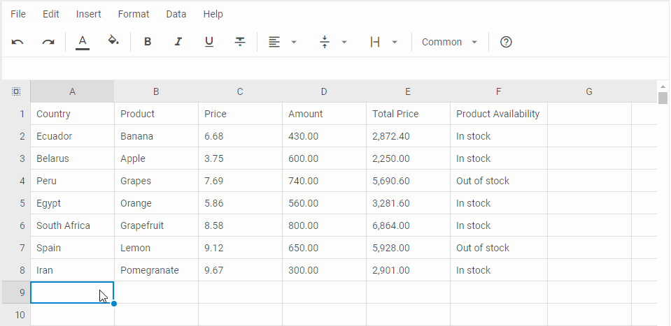
Merging and Splitting Cells
When manipulating different kinds of data in spreadsheets, it may be required to quickly change the grid structure. That is why we decided to bring in the ability to merge cells and split them back in v5.0. By merging cells, you combine two or more adjacent cells into a single one. It can be very useful for creating headings and labels or adding extra space for large pieces of content, thereby making it more readable.
In v5.0, end-users can merge any number of cells vertically or horizontally by simply selecting them and clicking on the Merge button in the toolbar. Alternatively, this feature is also available in the Format section of the spreadsheet menu.
You should also use one of the mentioned options if it becomes necessary to split the merged cell.
 Check the sample >
On the coding side, this functionality is enabled with the mergeCells() method. All you need to do is just specify a range of cells that should be merged in the first parameter.
The same method is used for splitting the merged cells. It is done by adding the second parameter with true as a value.
The new merged property in the sheet object aims to define a range of cells for merging.
Column Auto Width
Another helpful cell formatting feature shipped with v5.0 is automatic column width. It will help to forget about the necessity to manually change the width of any column when the content in its cells varies greatly in length.
In spreadsheets built with DHTMLX, end-users now can activate the automatic adjustment of a column to fit the longest content by a double-click on the column’s resizer or the context (3 dots) menu as follows:
 Check the sample >
Programmatically, you will be able to use this feature by applying the fitColumn() method. It takes one required cell parameter in which the ID of the needed column should be specified.
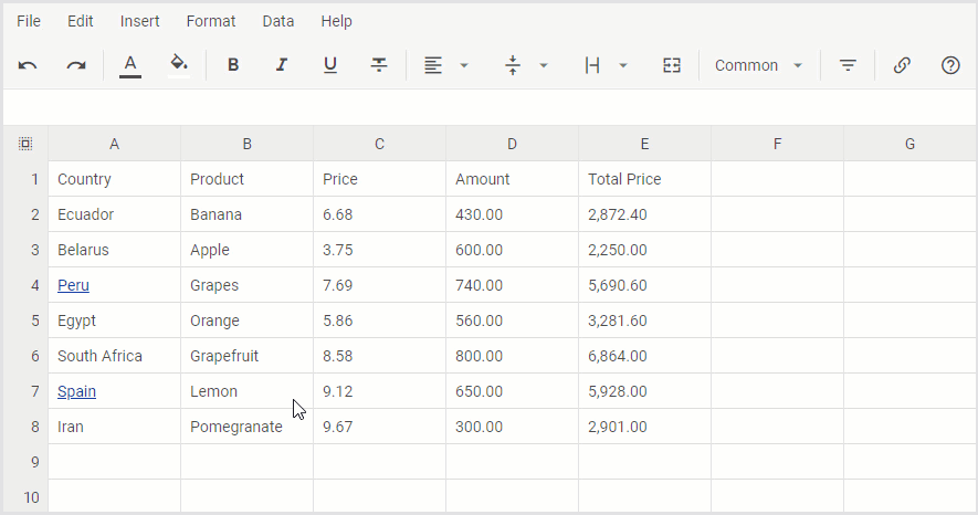
Hyperlinks in Cell Content
Starting from v5.0, cell content in DHTMLX-based spreadsheets may contain hyperlinks. It is common to use hyperlinks in cells to direct end-users to online documents or resources that are relevant to a given spreadsheet.
In practice, end-users are provided with three ways of inserting hyperlinks into cells:
- Insert link button in the toolbar
- hotkey combination (Ctrl (Command) + K)
- context menu of a cell
A cell with an embedded hyperlink will be complemented with a special popup, including three options for managing a link (copy, edit, remove).
 Check the sample >
In terms of coding, hyperlinks are inserted in a spreadsheet cell with the new insertLink() method. This method also allows adding a text (or numeric) value that will contain your hyperlink.
text:"DHX Spreadsheet", href: "https://dhtmlx.com/docs/products/dhtmlxSpreadsheet/"
});
Any hyperlink can be removed by calling the insertLink() method with the cell ID.
Other Changes and Updates
Let us finish with the main features of this release described above by mentioning some minor novelties related to them. First of all, there are new actions such as merge, unmerge, filter, fitColumn, and insertLink. In our JavaScript library, actions are used as a new way of interacting with spreadsheet events. The introduction of new capabilities in v5.0 also led to breaking changes in the toolbarBlocks property. Here we added a new toolbar block of controls named “actions” and replaced the “help” block with the “helpers” block.
Now we can proceed with other minor updates included in this release. There is a new text format called “Strikethrough“. It can be used for suggesting a revision in a particular cell by crossing out its content (or a part of it). It is put into play with the corresponding button in the toolbar or the hotkey combination Alt + Shift + 5 (Cmd + Shift + X).
 Check the sample >
And lastly, we also expanded the lists of available locales and hotkey combinations.
To make a quick revision of all new things packed in this release, visit the documentation page.
Take advantage of a free 30-day evaluation version to test the new DHTMLX Spreadsheet 5.0 in your own scenarios. Our current clients can download the latest version of our JavaScript spreadsheet component via their Client’s Area.
We are looking forward to your feedback on this major update in the comments below.